Magnolia is distributed with a variety of example models used to illustrate various aspects of the application’s operation. New users are encouraged to review the “Language Elements” examples in order to gain some familiarity with the modeling and scripting languages used by Magnolia.
- Language Elements
- Linearly Damped Forced Harmonic Oscillator
- Lorenz System
- Van der Pol Oscillator
- Bouncing Ball
- Spring/Pendulum System
- Control Loop
Language Elements
Basic Model Structure
When a new model file is created in Magnolia, the file contains some template code to help users get started. The template consists of a simple model for exponential decay, described by the differential equation:
\(\displaystyle\frac{dx}{dt} = -k x\)
This equation has an analytic solution, of course, but it provides a simple example of how a model is created in Magnolia:
- All model code is contained in an outermost section defined by the MODEL keyword (and a corresponding END statement). The MODEL keyword is followed by an identifier which provides a meaningful name for the model; this identifier should conform the to CSL variable naming conventions. Optional SUBMODEL (experimental) section may be placed ahead of the MODEL section to define reusable model components which may be instantiated in the MODEL section using the DIMENSION keyword
- Within the MODEL section are additional sub-sections denoted INITIAL, DYNAMIC, DERIVATIVE, DISCRETE and TERMINAL
- See the embedded comments for the meaning of each of the other section types
- Within the DISCRETE section are the equations related to the exponential decay model. In this case there are two equations: one defining the variable “x” as an ODE state which is computed by numerical integration, and another used to compute the value of the derivative
- The derivative also contains CONSTANT statements used to define model parameters. While these statements are placed in the DERIVATIVE section in this example, they actually can exist anywhere in the model code; their placement is generally a matter of preference. In some cases it may be clearer to place these statements in the INITIAL section, especially for large models
- The derivative also contains a TERMT statement, used to indicate the conditions under which the model should stop executing. Every model should contain at least one TERMT statement, which does not necessarily need to use a stopping time as the predicate. Some model, for example, terminate when one or more output values fall below a certain threshold, or when a particular kind of state crossing is detected.
- Although it contains no equations in this example, a DISCRETE section is included to illustrate their use. Generally, DISCRETE sections must have unique names, and are triggered using either a SCHEDULE statement or an INTERVAL statement.
- The DERIVATIVE sections and DISCRETE sections are contained in an enclosing DYNAMIC section. Strictly speaking this is not necessary, as the Magnolia translator automatically handles recognition of these sections regardless of where they appear in the model (they can even be embedded as nested sections within the initial or terminal sections). But placement within an enclosing DYNAMIC section is a typical coding practice.
|
1 2 3 4 5 6 7 8 9 10 11 12 13 14 15 16 17 18 19 20 21 22 23 24 25 26 27 28 29 30 31 32 33 34 35 36 37 38 39 40 41 42 43 44 45 46 47 48 49 50 |
! ! Magnolia CSL model file ! model Example initial ! The INITIAL section contains statements which are evaluated ! once at the beginning of the simulation run end ! initial dynamic ! The DYNAMIC section contains statements which are evaluated ! at each output time point derivative ! The DERIVATIVE section contains statements which are ! used to compute derivatives ! Example: exponential decay constant k = 1.0 ! Decay rate constant constant xic = 10.0 ! Initial condition xd = -k*x ! Derivative x = integ(xd, xic) ! Integrate derivative to compute state constant tstop = 10.0 termt(t >= tstop, 'Time limit') end ! derivative discrete DISCRETE_Example ! DISCRETE sections contain statements which are only ! evaluated at specific time points. A model ! can contain an arbitrary number of DISCRETE sections. end ! DISCRETE_Example end ! dynamic terminal ! The TERMINAL section contains statements which are evaluated ! once at the conclusion of the simulation run end end ! model |
Conditionals (if/else)
Conditionals in the CSL language are used to indicate the conditions under which certain statements/equations should be evaluated:
- Each branch of the conditional is denoted by the IF keyword, followed by a parenthesized logical expression (typically containing logical and/or relational operators)
- Alternative branches are denoted by the ELSE keyword, followed by another IF expression
- A default alternative is denoted by the final ELSE keyword in the overall conditional statement; the fact that the ELSE statement is not followed by another IF expression indicates that this is a default branch.
- The overall statement is terminated by the END keyword. Note that this differs from legacy implementation of the CSL language, in which a conditional was terminated with the ENDIF keyword.
|
1 2 3 4 5 6 7 8 9 10 11 12 13 14 15 16 17 18 19 20 21 22 23 24 |
model ConditionalExample derivative ! Conditionals are defined by sections of statements ! contained within "if", "else if" and "else" clauses. ! The conditional statement is now terminated with the ! "end" keyword if (t < 1.0) x = t^2 else if ( t < 1.35) x = exp(t) else if (t < 7.29) x = sin(t) else x = sqrt(t) end constant tstop = 10.0 termt(t >= tstop, 'Stopped on time limit') end ! derivative end ! program |
Loops
Iterating over a set of statements/equations (which typically involve array or matrix variables/constants) is accomplished with the FOR statement:
- The set of equations to be iterated over is delimited by the initial FOR statement and the enclosing END statement
- The FOR statement requires at least two arguments: the limits over which iterations should take place, and an optional step size.
- The iterator of the for statement can be an integer data type (used, for example, to index elements in an array), or a floating point value. The example below uses and integer value, which is declared via the DIMENSION statement just above the loop.
- For sitting purposes, the FOR loop is treated as a single statement; overall input and output dependencies are automatically detected by Magnolia. No sorting is performed within the FOR loop itself.
- If the FOR loop is not sorted as intended by default, it can be wrapped in a PROCEDURAL section to enforce an alternate sorting with respect to other statements in the model.
- FOR loops may be nested, and are allowed in any code section.
|
1 2 3 4 5 6 7 8 9 10 11 12 13 14 15 16 17 18 19 20 21 22 23 24 25 26 27 28 29 30 31 32 33 34 35 36 37 38 39 40 |
model LoopExample initial ! Declare an array that will be iterated over ! by a for loop ! Note that arrays are now declared and indexed using ! square brackets, not parentheses dimension resetTimes[5] constant resetTimes = 1.1, 2.8, 3.8, 4.93, 7.4343 constant ntimes = 5 ! The end of a loop statement is now denoted with the "end" ! keyword. Labeled statements and "continue" are no longer ! supported. ! The loop index shold be declared if it's an integer dimension integer i for i = 1, ntimes schedule reset at resetTimes[i] end end derivative constant k = 1.0 xd = k x = integ(xd, 0.0) constant tstop = 10.0 termt(t >= tstop, 'Stopped on time limit') end ! derivative discrete reset x = 0.0 end end ! program |
Discrete Events
Discrete events are sets of equations/statements that are to be executed at specific points in time (instantaneously), or when specific variables cross a threshold (so-called “state” events). In either case, the discrete even code has to be carefully synchronized with the continuous code. A time event, for example, may need to take place at a time which is not an even multiple of the simulation’s communication interval; thus, the simulation engine must know how to integrate up to the exact desired time, evaluate the discrete section code without advancing time, and then resume integration.
- Evaluation of code in a discrete section based on a specific time is accomplished via the SCHEDULE AT statement. The schedule statement require the name of the target discrete section and the value of time at which the section should be invoked. The time argument may be an arbitrary mathematical expression.
- SCHEDULE AT statements may be included in any section except the DERIVATIVE section.
- Handling of events on state crossings is done with the SCHEDULE XZ/XP/XN statement. This statement also accepts a section name and footing point expression as arguments. This type of SCHEDULE statement may only be used in the DERIVATIVE section.
- INTERVAL statements can be used as an alternative to SCHDULE AT statements when invocation of the discrete section needs to happen only at regular intervals. In this case the INTERVAL statement is included directly in the DISCRETE section it controls, with the syntax INTERVAL <variable name> = <interval length>.
|
1 2 3 4 5 6 7 8 9 10 11 12 13 14 15 16 17 18 19 20 21 22 23 24 25 26 27 28 29 30 31 32 33 |
model ScheduleExample initial schedule on at 0.0 schedule spike at 2.75 schedule spike at 5.03 schedule spike at 7.234 end derivative constant tstop = 10.0 termt(t >= tstop, 'Stopped on time limit') end ! derivative discrete on schedule off at t + 0.5 x = 1 end discrete off schedule on at t + 0.5 x = 0 end discrete spike x = 5 end end ! program |
Tables
In cases where it’s necessary to interpolate a continuous value from a list of tabulated x/y values, Magnolia provides the TABLE statement:
- The TABLE statement allows tabular 1, 2, or 3-dimensional data to be linearly interpolated based on a supplied value of an independent variable (or variables). The tabular independent and dependent data lists are supplied using array or matrix CONSTANTs.
- The TABLE statement essentially gives a name to the table for subsequent lookups, and assigned two or more CONSTANT arrays to the table name.
- Lookups (interpolations) of table values are performed by using the TABLE name as if it were a function call, supplying any required independent values as arguments.
- The CONSTANT arrays can be treated as any other constant values in CSL; that is, their values may be adjusted prior to runtime without need for recompilation of the model code.
|
1 2 3 4 5 6 7 8 9 10 11 12 13 14 15 16 17 18 19 20 21 22 23 24 25 26 |
model TableExample derivative ! The data which is to be interpolated via a TABLE statement ! is defined in 2 or more arrays ! Dimension the arrays dimension ageData[10], bwData[10] ! Populate the arrays with data constant ageData = 0, 1, 2, 3, 4, 5, 6, 7, 8, 9 constant bwData = 0.1, 0.13, 0.17, 2, 3, 5, 8, 11, 15, 20 ! Define the table. First arg after the equal sign is the ind var data table BodyWeightForAge = ageData, bwData ! This is where table lookups (interpolation) is done bw = BodyWeightForAge(t) constant tstop = 10.0 termt(t >= tstop, 'Stopped on time limit') end ! derivative end ! program |
Procedural Sections
In some cases, the default sorting of statements by Magnolia is not the sorting intended by the modeler. This sometimes happened with heavy use of array or matrix variables/constants. In these cases the input/out dependencies of a section of code may be explicitly specified for sorting purposes using the PROCEDURAL statement:
- The PROCEDURAL section looks somewhat like any other code section (it’s delimited by the PROCEDURAL and associated END keywords), with the exception that the PROCEDURAL keyword is followed by a parenthesized list of variable names.
- The variable names are arranged on either side of and equals sign. Variables on the left side of the equals sign are treated as outputs of the enclosed equations, for sorting purposes; variables on the right side are considered as inputs.
- The entire PROCEDURAL section is treated as a single statement, for sorting purposes, with the designated list of inputs and outputs replacing any input/output dependencies detected by Magnolia.
- PROCEDURAL sections are only necessary in DERIVATIVE section code, as that’s the only section where sorting in employed.
|
1 2 3 4 5 6 7 8 9 10 11 12 13 14 15 16 17 18 19 20 21 22 23 24 25 |
model ProceduralExample derivative dimension x dimension integer n constant L = 5, Pi = 3.1415927 ! Compute x using first 10 terms in Fourier series for square wave, ! Wrap the sum in a procedurak so that the value of x can be ! reinitilized to zero each time the sum is computed procedural(x = ) x = 0 for n = 1,19,2 x = x + (4/(Pi*n))*sin(Pi*n*t/L) end end constant tstop = 10.0 termt(t >= tstop, 'Stopped on time limit') end ! derivative end ! program |
Array Variables and Constants
It’s sometimes useful to create 1- 2- or higher-dimensional array/matrix variable for use in a model. This can happen for instance when:
- Using TABLE statements in a model
- Modeling quantities which are fundamentally multi-dimensional (e.g., position or velocity in 3-D space)
- When building finite-difference models within Magnolia to approximate phenomena which requires solution of a PDE
The syntax for declaration and element retrieval of an array variable or constant is straightforward, but differs a little from legacy CSL implementations:
- Arrays are defined using the DIMENSION statement, but the shape of the array is denote using square brackets instead of parenthesis
- Arrays are 1-based (not zero-based as ini many populate languages)
- Lookup (indexing, retrieval) of an array element is also performed using the square bracket notation
- Index values for accessing an element in an array must be integer values, and thus need to be declared as such using a DIMENSION statement.
- Array variables/constants can be used by the INTEG operator directly. Magnolia infers the shape of the argument to INTEG using the DIMENSION statements for the associated variables.
|
1 2 3 4 5 6 7 8 9 10 11 12 13 14 15 16 17 18 19 20 21 22 23 24 25 26 27 28 29 30 31 32 33 34 35 36 |
model ArraysExample derivative dimension x[2, 3], dx[2, 3], xic[2, 3], k[2, 3] constant xic = 0.1, 0.2, 0.3, 0.4, 0.5, 0.6 constant k = 1, 2, 3, 4, 5, 6 dimension integer i, j ! Wrap FOR loops in procedural to avoid any potential sorting errors procedural(dx = x) for i = 1, 2 for j = 1, 3 dx[i, j] = -k[i, j]*x[i, j] end end end ! The INTEG statement can be used on vector states, as long ! as both arguments are also vector values x = integ(dx, xic) constant tstop = 2.0 termt(t >= tstop, 'Stopped on time limit') ! Save array elements to scalars so they can be displayed in the interactive plot x11 = x[1, 1] x21 = x[2, 1] x12 = x[1, 2] x22 = x[2, 2] x13 = x[1, 3] x23 = x[2, 3] end ! derivative end ! program |
Functions
The FUNCTION statement is used to create reusable bits of code which can be evaluated using function-call notation, and which may or may not return a value. FUNCTION statements are somewhat similar to macro facilities in legacy versions of CSL. However, functions work in a different way than macros. While a macro is really a template for creating additional model code in the location where the macro is invoked, a function does not create additional code. Rather, it works like typical functions defined in most modern programming languages:
- The FUNCTION statement defines a set of statements/equations that an be repeatedly called from various places in model code
- FUNCTION statements include the specification of one or more optional input arguments, as well as an optional returned value
- Any variable used as an argument to a FUNCTION must be declared within the FUNCTION itself. These variables are shared with the rest of the model code, so care must be taken to avoid naming conflicts.
- User-defined functions are invoked in exactly the same way built-in CSL functions (or operators) are invoked.
|
1 2 3 4 5 6 7 8 9 10 11 12 13 14 15 16 17 18 19 20 21 22 |
model FunctionExample ! Definition of the function (genralized logistic function) ! Note: for now, these variables are shared with the rest of the ! model, so need to be careful of name conflicts function ss = genlog(aa, kk, bb, mm, nn, cc, tt) dimension aa, kk, bb, mm, nn, cc, tt ss = aa + (kk - aa)/((cc + exp(-bb*(tt - mm)))^(1/nn)) end derivative x1 = genlog(0, 1, 1, 5, 0.01, 1, t) x2 = genlog(0, 1, 1, 5, 0.1, 1, t) x3 = genlog(0, 1, 1, 5, 0.5, 1, t) constant tstop = 20.0 termt(t >= tstop, 'Stopped on time limit') end ! derivative end ! program |
Submodels (experimental)
SUBMODELs are an experimental feature of the modeling language used in Magnolia. One or more SUBMODEL sections may be specified in the model file before the main MODEL section. SUBMODELs are intended to be used when a set of equations representing identically modeled subsystems in a model can be “factored” out of the main model code. For example, one might imagine a model of an automobile which involves modeling four wheels. The wheels might each use the exact same model code, albeit with perhaps different parameters and coupled in a different way to the rest of the model. In Magnolia, the automobile model might be accomplished using a “Wheel” submodel, which includes four “Wheel” instances declared via a DIMENSION statement in main model, which might be called “Car.”
- One or more SUBMODEL sections can be introduced prior to the main MODEL section. Each SUBMODEL must have a unique name.
- One or more “instances” of each SUBMODEL are created in the main model using the DIMENSION statement, much in the same way one might declare an integer variable, or and array variable. Each “instance” is associated with a unique variable name.
- Variables belonging to each SUBMODEL are referenced from the main MODEL using “dot” notation. For example, to reference a variable called “omega” in a “Wheel” submodel from the main model, one would used the following syntax (assume the associated variable name in the main model is “wheel2”: foo = wheel2.omega.
- To override the values of constants defined in a SUBMODEL, additional CONSTANT statements are declared in the main model class which reference those constants using the “dot” notation. For example, if the “Wheel” model contains a constant named “radius”, the main model code might include a line like: CONSTANT wheel2.radius = 15.0
- When translating the model, Magnolia combines and sorts equations from the main model and all required submodels as necessary
|
1 2 3 4 5 6 7 8 9 10 11 12 13 14 15 16 17 18 19 20 21 22 23 24 25 26 27 28 29 30 31 32 33 34 35 36 37 38 39 40 41 42 43 44 45 46 47 48 49 50 51 52 53 54 55 56 57 58 59 60 |
! Model which clips output to fall within ! prescribed lower and upper bounds submodel Limiter constant lb = -1.0, ub = 1.0 function y = clip(x) dimension x if(x >= ub) y = ub else if(x <= lb) y = lb else y = x end end end ! Simple exponential decay model submodel Exponential derivative constant k = 1.0 constant xic = 1.0 xd = -k*x x = integ(xd, xic) end end ! Harmonic oscillator model submodel Harmonic derivative constant k = 1.0 constant xdic = 0.0, xic = 1.0 xdd = -k*x xd = integ(xdd, xdic) x = integ(xd, xic) end end ! Combined model model Combined initial constant kexp = 2.0, kharm = 3.0 m1.k = kexp m2.k = kharm end derivative dimension Exponential m1 dimension Harmonic m2 dimension Limiter m3 constant m1.k = 2.0, m2.k = 3.0 constant m3.lb = -0.5, m3.ub = 0.5 x1 = m1.x * m2.x x2 = m3.clip(x1) constant tstop = 10.0 termt(t >= tstop, 'Stopped on time limit') end end |
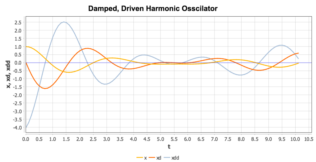
Linearly Damped, Forced Harmonic Oscillator
The motion of a (linearly) damped harmonic oscillator being driven by a force obeys the following equation of motion:
\(\displaystyle {m}{\frac{d^2x}{dt^2}}={F(t)}\, – {kx}\, – {c}{\frac{dx}{dt}}\)
where m is the mass of the object, F(t) is the driving force, c is the damping force coefficient, and k is the spring constant. For a sinusoidal driving force, this equation could be rewritten as:
\(\displaystyle {\frac{d^2x}{dt^2}}=({sin(\omega t)}\, – {kx}\, – {c}{\frac{dx}{dt}})\,/m\)
where omega is the angular frequency of the driving force.
To encode this in Magnolia, a few things need to be done:
- Variables need to be defined for the variable x, as well as its first and second derivatives; we’ll name these x, xd and xdd, respectively
- CONSTANT statements need to be created for any model parameters; well call these m, omega, c and k
- CONSTANT statements should also be defined for the initial conditions to be imposed on the state variables x and xd; in fact, literal numeric values could be placed in the INTEG statement, but this would make the model less flexible if initial conditions need to be adjusted
- INTEG statements need to be defined for the states x and xd; xdd is defined buy the equations above, while x and xd are defined by their INTEG statements
This results in a model like the following:
|
1 2 3 4 5 6 7 8 9 10 11 12 13 14 15 16 17 |
model HarmonicOscillator derivative constant c = 1.0, k = 10.0, omega = 2.0, m = 2.5 constant xic = 1.0, xdic = 0.0 xdd = (sin(omega*t) - c*xd - k*x)/m xd = integ(xdd, xdic) x = integ(xd, xic) constant tstop = 10.0 termt(t >= tstop, 'Time limit') end ! derivative end ! model |
Running this model results in the following trajectories for x, xd and xdd:
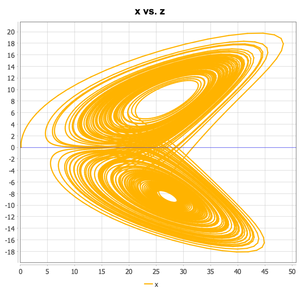
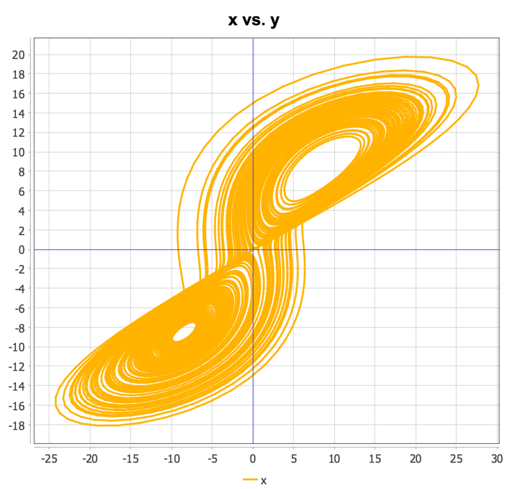
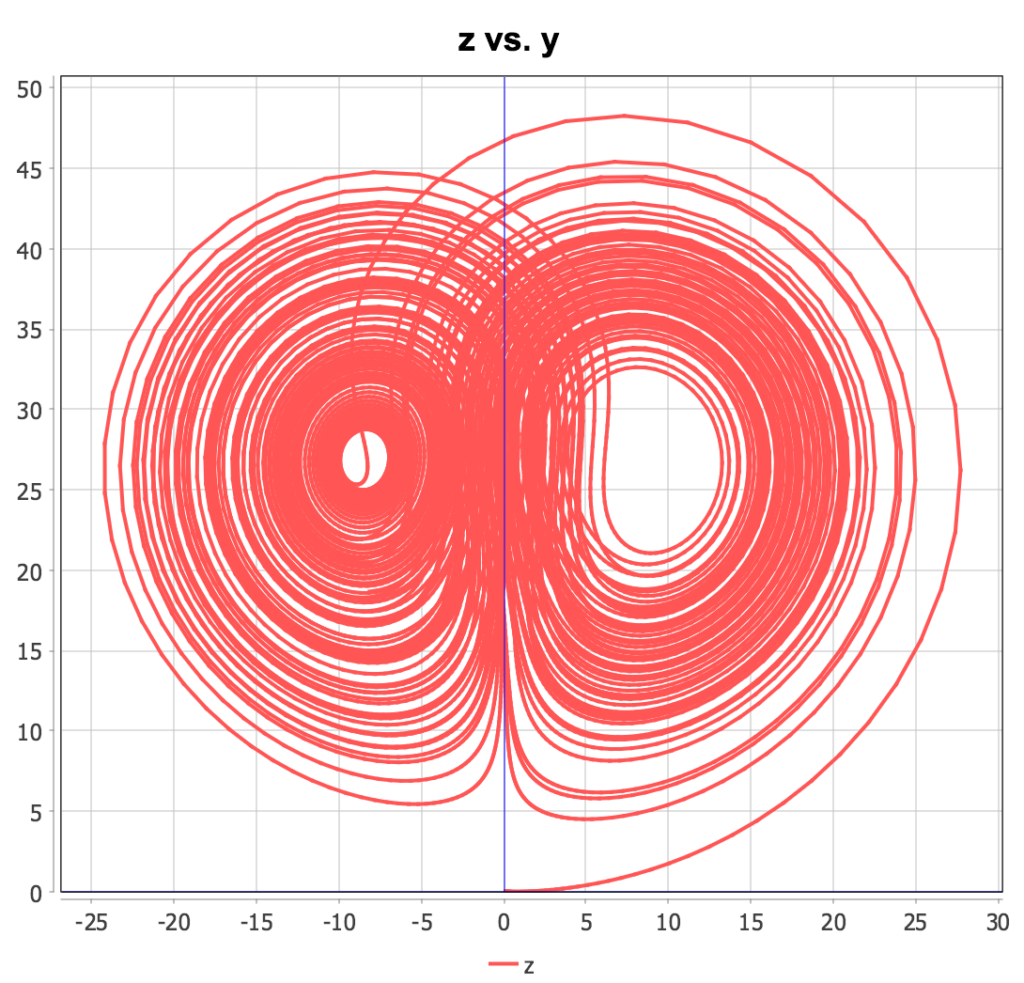
Lorenz System
The “Lorenz System,” originally created to model atmospheric convection, is defined by the following system of three first order coupled ODEs:
\(\displaystyle \frac{dx}{dt}=\sigma (y\, – x) \\  \displaystyle \frac{dy}{dt}=x (\rho\, – z)-y  \\ \displaystyle \frac{dz}{dt}=x y\, – \beta z\)
This system can be readily encoded in Magnolia as follows:
|
1 2 3 4 5 6 7 8 9 10 11 12 13 14 15 16 17 18 19 20 21 22 23 24 |
! Lorenz system model model Lorenz derivative ! Adjust the default output step size cinterval cint = 0.01 constant sigma = 10.0, rho = 28.0, beta = 2.6666666666666665 xd = sigma*(y - x) yd = x*(rho - z) - y zd = x*y - beta*z constant xic = 0.05, yic = 0.05, zic = 0.1 x = integ(xd, xic) y = integ(yd, yic) z = integ(zd, zic) constant tstop = 10.0 termt(t >= tstop, 'Time limit') end ! derivative end ! model |
This system is particularly interesting because of its chaotic behavior for certain choices of parameters. Two-dimensional “cross-sectional” plots of the solution trajectories can be constructed in a script such as this:
|
1 2 3 4 5 6 7 8 9 10 11 12 13 14 15 |
load 'lorenz.csl' ! Let Magnolia know which outputs need to be logged prepare t x y z ! Set tstop to a large number to generate lots of orbits set tstop = 100.0 ! Run the model start ! Generate "cross sections" of the trajectories plot @xvar=y z plot @xvar=y x plot @xvar=z x |
Running the above script produces the following plots:
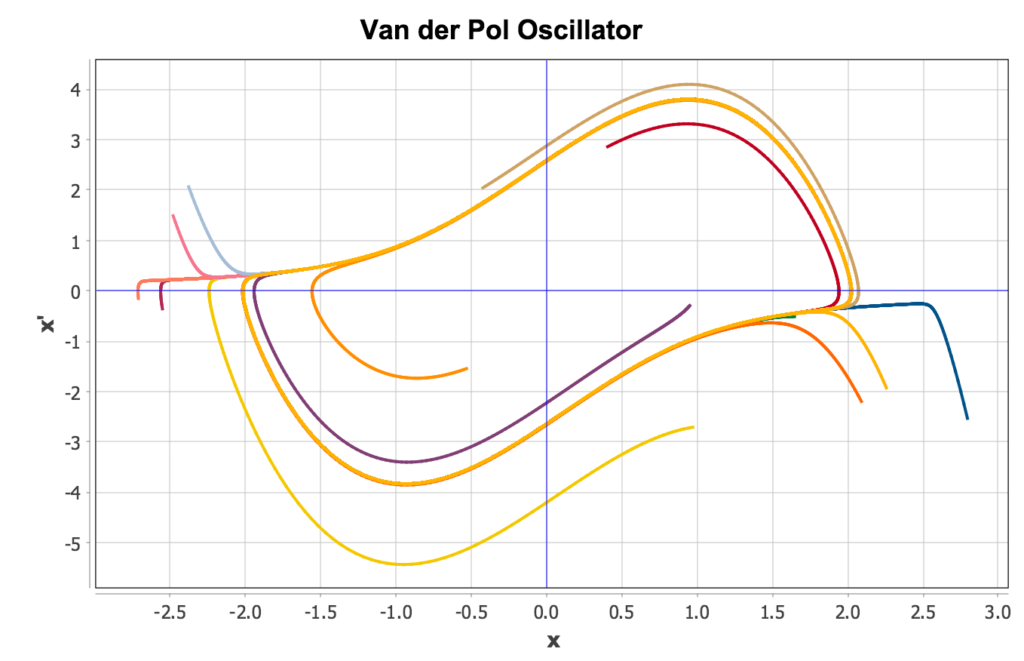
Van der Pol Oscillator
The Van der Pol oscillator is nonlinearly damped, nonconservative oscillator described by the following differential equation:
\(\displaystyle \frac {d^2 x}{dt^2}\, – \mu(1\, – x^2)\frac{dx}{dt} + x = 0\)
Solutions to the Van Der Pol equation display a “limit cycle” behavior. That is, the evolutions of solutions with difference initial conditions in phase space eventually reach the same stable orbit.
The Van der Pol differential equation can be simply encoded on Magnolia as follow:
|
1 2 3 4 5 6 7 8 9 10 11 12 13 14 15 16 17 18 |
model VanderPol derivative cinterval cint = 0.01 constant xic = -2.0, xdic = 4.0 constant mu = 2.0 xdd = mu*(1 - x^2)*xd - x xd = integ(xdd, xdic) x = integ(xd, xic) constant tstop = 10.0 termt(t >= tstop, 'Stopped on time limit') end ! derivative end ! model |
One way to illustrate the limit cycle behavior is to superimpose the solution trajectories from several runs using different initial conditions. The following Python script can accomplish this:
|
1 2 3 4 5 6 7 8 9 10 11 12 13 14 15 16 17 18 19 20 21 22 23 24 25 26 27 28 29 30 31 32 33 34 |
import math import random # Get a reference to the vanderpol model m = models.get("vanderpol.csl") # Set the prepare list m.prepare("t") m.prepare("x") m.prepare("xd") # Arrays into which conc trajectories will be placed xtrajs = [] xdtrajs = [] # Set the stopping time to something large, so we'll # collect enough output points for solutions to # converge to the limit cycle m.tstop = 100.0 # Iteration over random starting points for i in range(0, 15): m.xic = random.uniform(-3.0, 3.0) m.xdic = random.uniform(-3.0, 3.0) # Run the simulation m.run() # Append x and xd trajectories to local variables xtrajs.append(m.history("x")) xdtrajs.append(m.history("xd")) # Plot results h = plot.line(xtrajs, xdtrajs) |
Running this script produces the following plot:
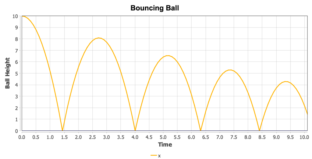
Bouncing Ball
This example models a bouncing ball falling under the force of gravity in one dimension and rebounding when hitting the floor with less than perfect elasticity. This requires using a state event (SCHEDULE XN) to detect the exact time when the ball hits the floor. At that instance, the ball’s velocity is negated and multiplied by a value of 0.9 to simulate the inelasticity f the collision:
|
1 2 3 4 5 6 7 8 9 10 11 12 13 14 15 16 17 18 19 20 21 22 23 24 |
model Bounce derivative schedule Bounce xn x constant xic = 10.0 constant xdic = 0.0 constant g = -9.8 xdd = g xd = integ(xdd, xdic) x = integ(xd, xic) constant tstop = 10.0 termt(t >= tstop, 'Stopped on time limit') end ! derivative discrete Bounce xd = -0.9*xd end end ! program |
Running the model above results in the following trajectory for x, the ball’s height:
Spring/Pendulum System
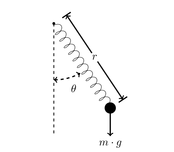
The combined spring/pendulum system is an interesting example in that a few equations of motion lead to very complex behavior in the dynamic system. In particular, phase plots (first derivative versus solution) can yield complex and fascinating designs. By creating an interactive phase plot using a CMD script, we can assign sliders to various model parameters, and watch these designs change interactively as the parameters are adjusted.
The equations of motion (translated to a system of first-order ODEs in polar coordinates) for the system are as follows:
\(\displaystyle\dot r = v_r \\ \dot \theta = v_\theta \\ \dot v_r = r {v^2_\theta} + g {cos(\theta)} – k(r – L) \\ \dot v_\theta = – \frac{(2 v_r v_\theta + g sin(\theta))}{r}\)
Where L is the equilibrium length of the pendulum, k is the spring constant, and g is the gravitational acceleration.
These equations can be directly implemented in a CSL model as follows:
|
1 2 3 4 5 6 7 8 9 10 11 12 13 14 15 16 17 18 19 20 21 22 23 24 25 26 27 28 29 |
model SpringPendulum ! Equations of motion explained here: ! https://ths.rwth-aachen.de/research/projects/hypro/spring-pendulum/ derivative constant g = 9.8, k = 2.0, L = 1.0 constant r0 = 1.2, theta0 = 0.5 constant vr0 = 0.0, vtheta0 = 0.0 cinterval cint = 0.02 rdot = vr thetadot = vtheta vrdot = r*vtheta^2 + g*cos(theta) - k*(r - L) vthetadot = -(2*vr*vtheta + g*sin(theta))/r r = integ(rdot, r0) theta = integ(thetadot, theta0) vr = integ(vrdot, vr0) vtheta = integ(vthetadot, vtheta0) constant tstop = 100.0 termt(t >= tstop, 'Time limit') end end |
To construct a phase plot, we can use the following simple script:
|
1 2 3 4 5 6 7 8 9 10 11 |
load 'spring_pendulum.csl' prepare t r rdot theta vr vtheta vthetadot start ! This is an example of how to create a slider-adorned interactive plot ! Note, this plot uses a variable other than time for the x-axis ! in order to create a phase plot. Fiddle with the sliders and ! watch it update interactively for hours of amusement. plot @interactive @xvar=vtheta vthetadot rdot r theta @param=k @param=l |
Running this script produces the following plot (before adjusting sliders all quantities plotted against theta):
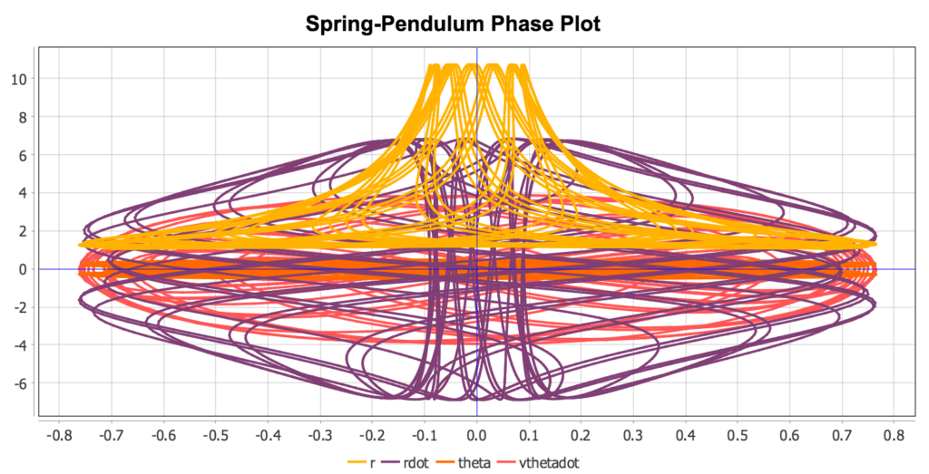
Adjusting the sliders will cause the plot to be interactively redrawn using the solutions with new parameter values. This can produce a variety of interesting phase plot “designs”.
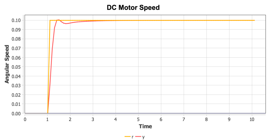
Control Loop
The Control Loop example illustrates the use of the SUBMODEL feature of CSL. This model is composed of a PID controller represented by one SUBMODEL, and a simple DC electric motor represented by a second SUBMODEL. These two submodels are connected in the main MODEL’s DERIVATIVE section:
|
1 2 3 4 5 6 7 8 9 10 11 12 13 14 15 16 17 18 19 20 21 22 23 24 25 26 27 28 29 30 31 32 33 34 35 36 37 38 39 40 41 42 43 44 45 46 47 48 49 50 51 52 53 54 55 56 57 58 59 60 61 62 63 64 65 66 67 68 69 70 71 72 73 74 75 76 77 78 79 80 81 82 |
! PID controller submodel Controller derivative ! The value of these variables will be set externally ! (they're inputs to this submodel) ! r = setpoint, desired vaue of y ! y = measured (actual) value of process variable dimension r, y ! error e = r - y ! PID controller gains constant Kp = 30.0, Ki = 50.0, Kd = 0.3 ! Derivative of error edint = integ(ed, 0.0) ed = (e - edint)/0.001 ! Integral of error eint = integ(e, 0.0) ! output u = Kp*e + Kd*ed + Ki*eint end end ! Simple electric DC motor model submodel Motor derivative ! Input: voltage dimension V constant J = 0.01, b = 0.1, K = 0.01, L = 0.5, R = 1.0 thetadd = (K*i - b*thetad)/J id = (V - K*thetad - R*i)/L thetad = integ(thetadd, 0.0) i = integ(id, 0.0) end end ! Combined motor + controller model model ControlLoop initial dimension Controller controller1 dimension Motor motor1 ! The statements are here purely to so we can set ! up sliders on an interactive plot constant Kp = 30.0, Ki = 50.0, Kd = 0.3 controller1.Kp = Kp controller1.Ki = Ki controller1.Kd = Kd end derivative ! Commanded value: target motor speed r = 0.1*step(1.0) ! Current motor speed y = motor1.thetad controller1.r = r controller1.y = y ! Command from controller u = controller1.u motor1.V = u constant tstop = 10.0 termt(t >= tstop, 'Stopped on time limit') end ! derivative end ! program |
An interactive plot can be created to enable “tuning” of the PID parameters using sliders with a simple CMD script:
|
1 2 3 4 5 6 7 |
load 'control_loop.csl' prepare t r y start plot @interactive r y @param=kp @param=ki @param=kd |
Running this script produces the following plot, which can be updated interactively by adjusting the sliders. By altering PID parameters, it’s possible to visually “tune” the PID controller to achieve optimal transient and stability characteristics.